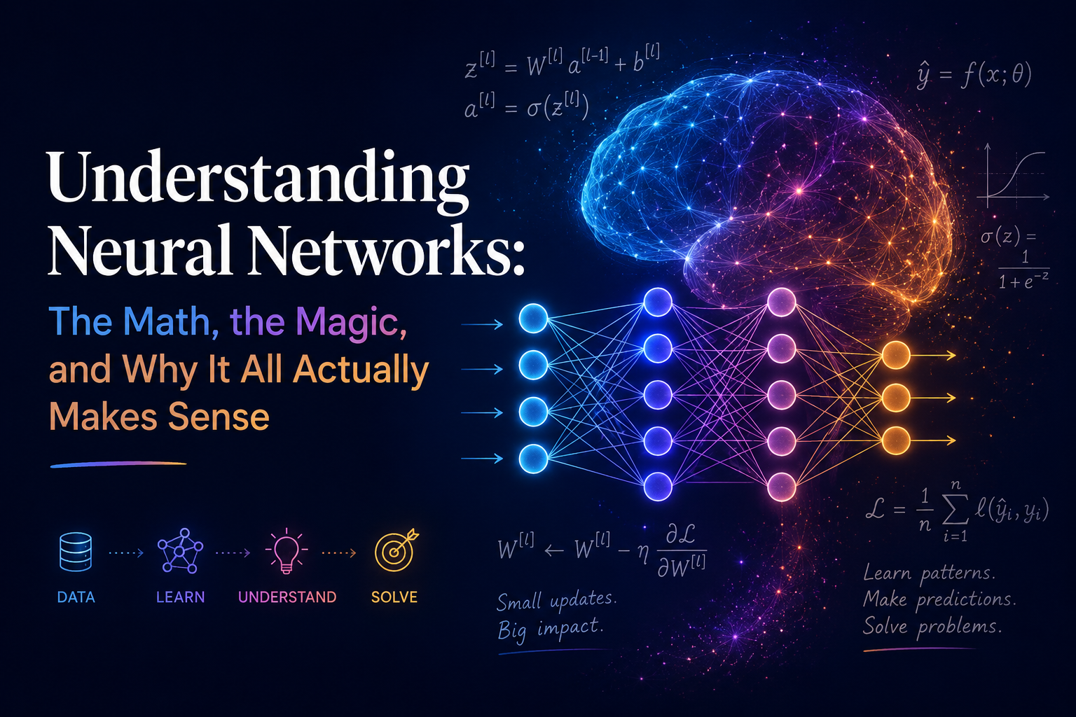
There’s a moment that nearly everyone hits when they first try to understand neural networks. You’re reading a blog post or watching a tutorial, everything’s going fine neurons, layers, yeah, makes sense and then someone drops a Greek letter into an equation and suddenly you feel like you’ve accidentally enrolled in a graduate-level mathematics course without your knowledge or consent.
Here’s the thing: that moment of confusion? Completely normal. And more importantly, completely survivable.
Neural networks sound intimidating because of how they’re talked about. “Deep learning.” “Backpropagation.” “Gradient descent.” The vocabulary alone creates a kind of velvet rope like there’s an exclusive club inside, and you need to know the password. But once you push past the jargon, what you find is actually a surprisingly elegant set of ideas. Ideas that, when you see them clearly, make you think: oh. That’s it? That actually makes sense.
This article is your guided walk through those ideas the math, the intuition, and the real-world relevance. No PhD required.
What Is a Neural Network, deep learning basics Really?
Let’s start not with a textbook definition, but with something more useful: an analogy that holds up.
Imagine you’re teaching a child to recognize dogs. You don’t sit them down and write out a rulebook “four legs, fur, tail, barks.” You just show them dogs. Hundreds of them. Big dogs, small dogs, fluffy dogs, short-haired dogs. Over time, the child builds up an internal model of what “dog” looks like, one that’s flexible enough to handle a Chihuahua and a Saint Bernard as members of the same category.
A neural network does something structurally similar. It learns from examples rather than from explicit rules. You feed it thousands of labeled images “this is a dog,” “this is not a dog” and it adjusts its internal parameters until it gets reliably good at telling the difference deep learning basics
The “neural” part of the name comes from a loose analogy to biological neurons in the brain. Real neurons receive signals, process them, and fire if the signal is strong enough. Artificial neurons do something mathematically similar: they receive inputs, multiply each by a weight (a measure of importance), add them up, and pass the result through a function that decides how strongly to “activate.”
That’s it. That’s the core idea. Everything else the deep architectures, the sophisticated training algorithms — is built on top of this simple foundation.
The Architecture: Layers Upon Layers
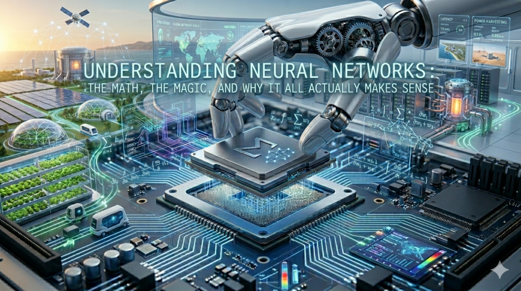
A neural network is organized into layers. Picture a flowchart that goes left to right.
| Layer Type | Position | Role |
|---|---|---|
| Input Layer | Far left | Receives raw data — pixels, numbers, text tokens |
| Hidden Layers | Middle | Detects increasingly abstract features |
| Output Layer | Far right | Produces the final answer or prediction |
On the far left is the input layer this is where raw data enters. If you’re working with an image, each pixel becomes a number (usually representing color intensity from 0 to 255), and each of those numbers is one input node.
On the far right is the output layer this is the network’s answer. For a dog/not-dog classifier, you’d have two output nodes: one representing the probability it’s a dog, one for the probability it isn’t.
In between are the hidden layers, and this is where the interesting work happens. Each hidden layer learns to detect increasingly abstract features. The first layer might pick up on edges and color gradients. The second layer might combine those into shapes curves, textures. Deeper layers might recognize ears, snouts, tails. The final layer combines all of that into a confident classification.
This layered structure is what “deep learning” refers to networks with many hidden layers. “Deep” just means deep in layers, not deep in some philosophical sense (though the results sometimes feel like magic, which earns the word a little poetic license).
Where the Math Lives: Weights, Biases, and Activation Functions
Okay. Here’s where we get into the numbers. Don’t panic we’re going to take this slowly, and by the end, you’ll see why this particular math was chosen deep learning basics.
Weights and the Dot Product
Every connection between neurons has a weight a number, positive or negative, that represents how much influence one neuron has on the next. If a weight is large and positive, that connection strongly activates the next neuron. If it’s negative, it suppresses it.
When a neuron receives its inputs, it computes a weighted sum: multiply each input by its corresponding weight, then add all those products together. In matrix notation which is how computers actually compute this you’re doing a dot product between the input vector and the weight matrix.
If you’ve ever taken a linear algebra class, you’ve seen this before. If you haven’t, the intuition is simpler than the notation suggests: it’s just a structured way of saying “add up all the influences, scaled by importance.”
Biases: The Offset You Didn’t Know You Needed
Along with weights, each neuron also has a bias a number added to the weighted sum before activation. Think of it as the neuron’s default disposition. A high bias means the neuron is more likely to activate even when inputs are weak. A low bias means it needs a stronger signal.
Mathematically: output = activation(weights · inputs + bias).
The bias gives the network more flexibility. Without it, every decision boundary the network could draw would have to pass through the origin a severe and arbitrary constraint. With it, the network can shift its decisions to fit the data far more naturally.
Activation Functions: Injecting Non-Linearity
Here’s a subtle but critical point. If all a neural network did was multiply inputs by weights and add biases, the entire network no matter how many layers would collapse into a single linear transformation. You could represent the whole thing with one matrix multiplication. All that depth would be mathematically meaningless.
What breaks this is the activation function a nonlinear function applied to each neuron’s output before it passes to the next layer. Here’s how the most common ones compare:
| Activation Function | Formula | Output Range | Best Used For |
|---|---|---|---|
| ReLU | max(0, x) | 0 to infinity | Hidden layers; fast training |
| Sigmoid | 1 (1 + e^-x) | 0 to 1 | Binary output probabilities |
| Tanh | (e^x – e^-x) (e^x + e^-x) | -1 to 1 | Centered data; RNNs |
| Softmax | e^xi sum(e^xj) | 0 to 1 (sums to 1) | Multi-class output layer |
The most commonly used one today is ReLU (Rectified Linear Unit): f(x) = max(0, x). It’s almost comically simple: if the input is negative, output 0. If positive, output it unchanged. But this tiny nonlinearity, repeated across thousands of neurons and dozens of layers, gives neural networks the capacity to approximate almost any function a property known as the Universal Approximation Theorem.
ReLU became dominant because it trains faster and avoids a problem called the “vanishing gradient” — more on that in a moment.
How Networks Learn: Backpropagation and Gradient Descent
Here’s where many explanations lose people, and it’s a shame, because the learning algorithm is actually one of the most beautiful parts of the whole thing.
The Loss Function: Measuring How Wrong You Are
Before a network can learn, you need a way to measure how wrong its current answers are. That’s the loss function (sometimes called a cost function).
| Problem Type | Common Loss Function | What It Measures |
|---|---|---|
| Binary classification | Binary cross-entropy | Gap between predicted and actual probability for 2 classes |
| Multi-class classification | Categorical cross-entropy | Gap across multiple class probabilities |
| Regression | Mean Squared Error (MSE) | Average squared difference between prediction and true value |
| Object detection | Focal loss | Emphasizes hard-to-classify examples |
For classification problems, cross-entropy loss measures the gap between the network’s predicted probability distribution and the actual distribution. For regression problems, mean squared error averages the squared differences between predictions and true values.
The loss is a single number. A high loss means the network is badly wrong. A low loss means it’s doing well. Training is the process of pushing this number down.
Gradient Descent: Rolling Downhill
Imagine the loss function as a landscape of hills and valleys. Your current weights put you at some point on that landscape. You want to reach the lowest valley minimum loss but you can’t see the whole map. What can you do?
You look at the slope beneath your feet and take a step downhill.
That’s gradient descent. The gradient is the mathematical direction of steepest increase in the loss function. Move opposite to it downhill and you reduce the loss. Take small steps in this direction repeatedly, and you eventually reach a (local) minimum.
The size of each step is controlled by the learning rate one of the most important hyperparameters in deep learning. Too large a learning rate, and you overshoot valleys and bounce around without settling. Too small, and training takes forever. Finding the right learning rate is part art, part science.
Backpropagation: Distributing Credit
Here’s the clever part: how do you know which weights to adjust?
Backpropagation is the algorithm that computes the gradient of the loss with respect to every single weight in the network, efficiently. It works by applying the chain rule of calculus a rule that says if you want to know how one thing affects another thing through an intermediary, you multiply the rates of change at each step.
Starting from the loss, the algorithm propagates gradients backward through the network layer by layer, computing each weight’s contribution to the final error. It’s computationally elegant: what would naively require enormous computation for a large network can be done efficiently because information from earlier computations is reused at each step.
The result is a gradient for every weight in the network a readout of exactly which direction to nudge each parameter to reduce loss.
The Vanishing Gradient Problem
One challenge that plagued early deep networks is the vanishing gradient problem. When gradients are propagated backward through many layers, they’re repeatedly multiplied by the derivatives of activation functions. For sigmoid and tanh functions, these derivatives are small numbers less than 1. Multiply enough small numbers together, and the gradient shrinks to nearly zero before it reaches the early layers.
When gradients vanish, early layers stop learning. The network gets stuck. ReLU largely solved this: its derivative is just 1 for positive inputs, so gradients flow through without shrinking. This is one major reason ReLU transformed deep learning when it was popularized around 2010.
From Theory to Reality: What Neural Networks Actually Do
All of that math produces something remarkable in practice. Here’s how it maps onto applications you’ve probably already encountered:
| Application | What the Network Learns | Example |
|---|---|---|
| Image recognition | Edges, shapes, textures, objects | Google Photos, medical imaging |
| Language models | Grammar, context, meaning, reasoning | ChatGPT, Claude, Gemini |
| Drug discovery | Molecular interaction patterns | Predicting protein folding (AlphaFold) |
| Recommendation systems | User preference patterns | Netflix, Spotify, YouTube |
| Fraud detection | Unusual transaction patterns | Bank card security systems |
| Speech recognition | Phoneme and word patterns | Siri, Alexa, Google Assistant |
Image recognition. When a neural network classifies images, it’s learning a hierarchy of visual features textures, shapes, objects through nothing but gradient descent on labeled examples. The same basic architecture powers everything from photo apps on your phone to medical imaging systems that detect tumors.
Language models. The large language models reshaping the tech industry including the one that might have appeared suspiciously helpful to you recently are neural networks at heart. They’re far more complex, using architectures called transformers with attention mechanisms, but they learn from data using the same fundamental backpropagation algorithm.
Drug discovery. Pharmaceutical companies use neural networks to predict how molecular structures will interact with biological targets dramatically speeding up the identification of drug candidates. The math of weighted sums and gradient descent turns out to generalize across very different domains.
Recommendation systems. When Netflix suggests a show or Spotify generates a playlist that’s uncannily right for your mood, that’s neural network-based collaborative filtering working behind the scenes, having learned patterns from millions of users’ behavior.
A Few Things Neural Networks Can’t Do (That People Often Assume They Can)
It would be dishonest to write an enthusiastic explanation of neural networks without noting their real limitations.
| Limitation | What It Means in Practice |
|---|---|
| No true understanding | Networks find statistical patterns, not meaning. They can fail strangely on inputs that differ from training data. |
| Data hungry | Strong results usually require massive labeled datasets that are expensive to collect and curate. |
| Computationally costly | Training large models requires significant GPU resources and energy — GPT-scale training costs millions of dollars. |
| Opaque decisions | It’s often very hard to explain why a network made a specific prediction — a serious issue in high-stakes settings. |
| Brittle under distribution shift | A model trained on sunny-day photos may underperform in rain or fog. |
Neural networks don’t “understand” in the way humans do. They find statistical patterns in training data. When those patterns break down when inputs look very different from the training distribution networks can fail in ways that feel bizarre to humans. An image classifier that performs brilliantly on clear photos might fall apart with slight lighting changes or adversarial perturbations invisible to the human eye.
They’re also hungry for data. The impressive results you read about usually required massive labeled datasets and significant computational resources. Training GPT-scale models costs millions of dollars. That’s not a deterrent from learning about the field, but it’s worth knowing the full picture.
And they’re opaque. This is a genuine active research problem. When a neural network makes a decision, it’s often very hard to explain why which matters enormously in high-stakes settings like medical diagnosis or loan approval. The field of explainable AI (XAI) is working on this, but it remains unsolved.
Where to Go From Here

If you’ve read this far and feel a click of genuine curiosity, the good news is that the barriers to going deeper are lower than ever.
| Resource Type | Tool or Platform | What It Offers |
|---|---|---|
| Libraries | PyTorch, TensorFlow, Keras | Build and train neural networks in Python |
| Free compute | Google Colab, Kaggle Notebooks | GPU access in the browser, no setup needed |
| Courses | fast.ai, deeplearning.ai | Practical and theory-first approaches |
| Math foundations | Khan Academy, 3Blue1Brown | Linear algebra and calculus, explained visually |
| Books | “Deep Learning” by Goodfellow et al. | Comprehensive academic reference, free online |
The math isn’t optional if you want to go deep (the pun is unavoidable). Linear algebra particularly matrix operations and eigenvalues is the core language. Calculus, specifically the chain rule and partial derivatives, is essential for understanding backpropagation. Probability theory becomes important when you’re thinking about loss functions and model uncertainty. These aren’t weekend reads, but they’re not impenetrable either, especially with the wealth of free, well-taught resources available today.
Start somewhere. Build something small that does something you care about. The math becomes far less abstract once it’s attached to a problem you actually want to solve.
The Bigger Picture
Neural networks are not magic, even when they produce results that feel magical. They’re function approximators machinery for learning mappings from inputs to outputs by optimizing mathematical objectives over large amounts of data. The math is real, the tradeoffs are real, and the limitations are real.
But within those constraints, they’re also genuinely extraordinary. The idea that a relatively simple optimization process, applied at scale, can teach a computer to recognize faces, translate languages, generate images, and reason about text that’s still, even after years of following this field, kind of astonishing.
Understanding how it works doesn’t diminish the wonder. If anything, it deepens it. The more clearly you see the machinery the weighted sums, the chain rule, the loss landscapes the more impressive the outcomes become, precisely because you understand what’s not there. There’s no magic ingredient. Just math, data, and a lot of careful engineering.
And the ability to understand it is well within your reach. Start with the intuition. Follow with the math. Build something. The velvet rope was never locked to begin with.
Have questions about specific neural network architectures or the math covered here? Drop them in the comments — the best learning often happens in the conversation after the article.
FAQ
Q: What exactly is a neural network in simple terms?
A neural network is a computer system loosely inspired by the structure of the human brain. It processes information through layers of connected mathematical nodes, each one passing signals forward and adjusting based on what it learns from data. Rather than following hand-coded rules, it learns patterns by example — seeing thousands of inputs, making predictions, measuring how wrong those predictions were, and adjusting until it gets reliably good at the task.
Q: Why are they called “neural” networks?
The name comes from biological neurons — the cells in your brain that fire electrical signals to each other across trillions of connections. Artificial neural networks borrow that basic architecture: many simple units, each connected to others, collectively producing complex behavior that no single unit could achieve alone. The analogy has limits (artificial neurons are far simpler than biological ones), but the core inspiration — layered, connected processing — is genuine.
Q: What’s the difference between a neural network and regular programming?
In traditional programming, a human writes explicit rules: “if this condition, do that action.” A neural network doesn’t receive explicit rules. Instead, it receives examples — thousands or millions of them — and learns the rules implicitly by identifying statistical patterns across those examples. The difference matters most in tasks where the rules are too complex to write down, like recognizing a face or understanding a sentence spoken with an accent.
How Neural Networks Learn
Q: How does a neural network actually learn from data?
Through a cycle called training. The network receives a labeled example, makes a prediction, and a function called the loss function measures how far off that prediction was. That error signal then travels backward through the network — a process called backpropagation and an algorithm called gradient descent makes tiny adjustments to the weights connecting each node. Repeat this millions of times across millions of examples, and the weights gradually settle into values that produce accurate predictions.
Q: What are weights and biases, and why do they matter?
Every connection between nodes in a neural network has a numerical value called a weight, which determines how much influence one node has on the next. Biases are additional adjustable values that shift the activation threshold of a node. Both are tuned during training. After enough iterations, the weights and biases encode the pattern the network has learned they’re what the network “knows,” stored numerically rather than as words or rules.
Q: What is backpropagation?
Backpropagation is the algorithm that makes training deep neural networks computationally feasible. After a forward pass where data flows through the network and produces a prediction — the resulting error flows backward through every layer. Using the calculus chain rule, the algorithm computes exactly how much each individual weight contributed to the mistake. Those contributions are then used to update the weights in the right direction. Without backpropagation, there’d be no efficient way to train a network with millions of parameters.
Q: What is gradient descent?
Gradient descent is the optimization algorithm that does the actual weight-updating during training. Imagine standing blindfolded on a hilly landscape and trying to find the lowest valley — you’d feel the slope under your feet and take a step downhill, then repeat. Gradient descent does the same thing mathematically: it calculates which direction is “downhill” in the loss function, and nudges the network’s weights one step in that direction. Repeat enough times, and the network converges toward a configuration that minimizes its errors.
Q: What is the learning rate, and why does it matter?
The learning rate controls how large each step is during gradient descent. Too large, and the network overshoots the optimal solution and bounces around erratically — loss can actually increase instead of decreasing. Too small, and training crawls painfully, sometimes getting stuck before making meaningful progress. Finding the right learning rate is one of the first things practitioners tune when training a model, and techniques like learning rate schedules (gradually reducing it over time) help manage this throughout training.
Architecture and Types
Q: What does “deep” mean in deep learning?
It refers to depth — how many hidden layers a neural network has between its input and output. A shallow network might have one or two hidden layers. A deep network might have dozens, hundreds, or even thousands. More depth generally allows the network to learn more complex, abstract, and hierarchical patterns. A deep image recognition network might learn edges in the first layer, shapes in the next, object parts further on, and whole objects in the deepest layers.
Q: What’s the difference between a hidden layer and an output layer?
Every neural network has three types of layers. The input layer receives raw data. Hidden layers — there can be one or many — transform that data through successive rounds of weighted computation, extracting increasingly abstract features. The output layer produces the final answer: a classification, a probability score, a generated text token, or whatever the task requires. The “hidden” in hidden layers simply means they’re internal to the network — neither receiving the raw input nor producing the final output.
Q: What is a Convolutional Neural Network (CNN)?
A CNN is a specialized architecture designed for processing grid-structured data, most commonly images. Instead of connecting every node to every other node, CNNs apply small learnable filters that slide across the input, detecting localized features like edges, textures, and shapes. Successive layers combine these local features into increasingly complex representations. CNNs are the architecture behind facial recognition, medical image analysis, and most computer vision applications.
Q: What is a Transformer, and why does it matter?
The Transformer, introduced in a 2017 paper titled “Attention Is All You Need,” is the architecture behind most modern language AI — GPT, BERT, Claude, and the models powering search and translation at scale. Its key innovation is an attention mechanism that allows every part of an input to directly influence every other part simultaneously, rather than processing information sequentially. This solved the long-range dependency problem that plagued earlier architectures and made large-scale language modeling practical.
Read about Discover the math